Week 4: Debug & Basic design of poster

There are five tasks for this week.

1.     Achieving the coding of position of sink (base station).

2.     Comparing the performance of three protocols.

3.     Collecting the number of data packets of each nodes.

4.     Considering the diversity of the solar energy for each node.

5.     Working on design the poster and obtain the basic frame of poster.

After discussing with supervisor, the diversity of solar energy had been solved. The diversity means that for different nodes in various position, the collection efficiency for each nodes is different. Thus, in the beginning of the program, a random percentage is produced for total solar energy of each sensors.

Last week, the method of determining the position of sink was achieved. This week, the coding is compiled successfully. The main way is to find the minimum number of connection hops. This week, the lifetime of three protocols is compared. However, optimizing solution based on SPIN has some problems due to the lifetime is less than time of gossiping.

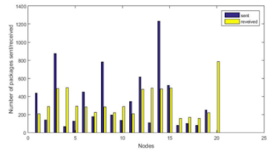
For better observing the behavior of each nodes, the number of data packets of each nodes is visualized by histogram which is shown below.

Figure 1: the number of data packets of each node

Meanwhile, the fundamental knowledge which is called WSN OSI LAYER for this project is introduced. There are five layers for wireless sensor networks and each layer has specific functions.

• Physical layer
• Application layer
• Transport layer
• Network layer
• Data link layer

The main layer is physical layer and its function is to provide interface to transmit steam of bits. The existence of transport layer is for deciding the protocol. The coding and operation of whole program is based on this basic principal knowledge.

In addition, the frame of poster is designed and the rough layout is shown below.

Figure 2: the first layout of poster

Final week, the main object is to debug three touting protocols and achieve final design of poster. In addition, we will prepare for bench inspection in Week 6 and discuss some possible questions.

Week 3: Improvement of protocols

Last week, the coding of two routing protocols (FLOODING & GOSSIPING) were compiled. After discussing with supervisor, the obtained results were right and there were some problems. First, the sink (base station) should be added to the sensor nodes system for collecting whole energy. Secondly, the figure only shows that the energy was consumed and we need to show the increasing of energy for achieving the sustainable operation and extending the lifetime of system.

This week, several parts had been finished.

1.    The values of various parameters were specified. For instance, battery capacity and energy consuming when sensor transmit or receive data packets. There are two equations which are used for calculating the energy.

• §  For transmission of data: E=E(elec) + C(amplification)d², E(elec) is a constant which is communication module, C(amplification) represents amplification constant. The data should be amplified when it is transmitted and d means the distance between two nodes.
• §  When the sensor receiving the data packet, the data need not to be amplified and the energy is only equal to the energy of communication module. Thus the equation is E=E(elec).

2.    The program for optimizing solution based on flooding protocol was coded.

3.    The sink (base station) was fixed and the best position was built.

4.    The lifetime between flooding and optimizing solution based on flooding protocol was compared. For accelerating the run time of program, the size of data packets was enlarged 100 times. Finally, the rough result for optimized solution is 7 days and 60000 seconds, while for flooding, the lifetime is 2 days and 60000 seconds.

The optimizing solution is based on SPIN (sensor protocols for information via negotiation) protocol. When a sensor has data that want to transmitted, it will send a broadcast signal which called ADV to its neighbors, and then the neighbors who has no data can send a signal called REQ back. Final, the node which receive the REQ signal will transmit data packets. In addition, for extending the lifetime of system, there is a judgmental statement of time. If a sensor node of a hop has very low power, this statement will work to calculate the time for another hops without low power node. If the time is less than a specific value, it means that another hop can work and the data packets are transmitted to destination node. In contrast, the hop will work although the node has low power.

For determining the position of sink (base station), a possible method was provided. First, middle point of distribution is determined, which mean the number of node for a hop is minimum. In addition, if there are several middle point node, middle point of distance will be considered. Then the only one distribution node is chose based on the minimum distance between middle distribution nodes and middle distance node. However, the coding of this method had not been compiled successfully. This problem will be solved next week.

Week 2: The coding of first routing protocol——Flooding

After the basic arrangement of the group in last week, the group began to code main program. On Tuesday, we summarized the activities and achievements for our academic supervisor in tutorial meeting, and then we determined that our general recognition of project is right. In addition, basic solution of how to connect all nodes for ensuring the sensors network connectivity was formed, which is to build a matrix and each element represents whether two nodes are connected and Logic 1 means connection. In addition, the supervisor advised that we need to generate the diagram of sensors connectivity, which is convenient for judge whether all nodes are connected in system.

Firstly, the fundamental definition of flooding was determined. Flooding is an old technique for sensor network, it requires node to transmission the data package to their neighboring nodes and the transmission will stop until the data is received by the goal node. Another three routing protocols are based on flooding, thus the program should be began from flooding for high work efficiency. For better understanding the flooding, the diagram of communication between sensors network is shown below.

Figure 1: the working diagram of Flooding

According to the advice of supervisor, an adjacency matrix is achieved for judging if two codes in system are connected. The specific code is shown below.

function main()
a0 =     0.09222;
a1 =    -0.02355;
b1 =     -0.1881;
a2 =    -0.08995;
b2 =     0.02183;
a3 =   5.342e-05;
b3 =    0.008936;
a4 =    -0.01734;
b4 =     0.01367;
a5 =    0.008954;
b5 =    0.008516;
w =      0.3664;
date = 0; %%initialize date
time = 0; %%~ time(in second, 0 to 3600*24 for each day)
totalNode = 16;
sensorArray = cell(1,totalNode);
delivered = 0; totalDev = 0;
distMatrix = zeros(totalNode,totalNode);%%
adjMatrix = zeros(totalNode,totalNode);%%
cMatrix = zeros(totalNode,totalNode);
XY = zeros(totalNode,2);  %%these three variables are used to draw adjacency graph
connected = 0;
connectCounter = 0;
for num = 1:1:totalNode
x = unifrnd(0,25);
y = unifrnd(0,25);
sensorArray(num) = {sensorNode(num,num,x,y)}; %%construct the nodes
end
from = randi([1,totalNode],1);  %%generate a node which transmit data
to = randi([1,totalNode],1)  %%generate some nodes which are objective nodes
%%plot the 3d graph
for i = 1:1:totalNode    %% construct the sensor array
XY(i,1) = sensorArray{i}.x;
XY(i,2) = sensorArray{i}.y; %%define the axis
for j = 1:1:totalNode
distMatrix(i,j) = sqrt((sensorArray{i}.x-sensorArray{j}.x)^2 + (sensorArray{i}.y-sensorArray{j}.y)^2);
if distMatrix(i,j) < 10 && distMatrix(i,j) ~= 0
adjMatrix(i,j) = 1;  %%generate adjacency matrix
sensorArray{i} = sensorArray{i}.addSubnode(sensorArray{j});  %%for any node that can be reached, add it as bunNode
sensorArray{j} = sensorArray{j}.addSuper(sensorArray{i});
end
end
end
cMatrix = conMatrix(adjMatrix,totalNode);
cMatrix2 = cMatrix;
for i = 1:1:totalNode
plot3(sensorArray{i}.x,sensorArray{i}.y,0,'*');
hold on;          %plot all the points
cMatrix2(i,i) = 1;  %cpy
end
for i = 1:1:totalNode
for j = 1:1:totalNode
if cMatrix2(i,j) ~= 0
connectCounter = connectCounter + 1
end
end
end
if connectCounter == totalNode^2
connected = 1;
end
if connected == 0
disp('the network cannot be connected');
end
while connected == 1  %%start of while
allHaveEnergy = 0;
time = time + 900
t = (time)/3600;
power =  a0 + a1*cos(t*w) + b1*sin(t*w) + a2*cos(2*t*w) + b2*sin(2*t*w) + a3*cos(3*t*w) + b3*sin(3*t*w) + a4*cos(4*t*w) + b4*sin(4*t*w) + a5*cos(5*t*w) + b5*sin(5*t*w);
power1 = a0 + a1*cos((t+0.25)*w) + b1*sin((t+0.25)*w) + a2*cos(2*(t+0.25)*w) + b2*sin(2*(t+0.25)*w) + a3*cos(3*(t+0.25)*w) + b3*sin(3*(t+0.25)*w) + a4*cos(4*(t+0.25)*w) + b4*sin(4*(t+0.25)*w) + a5*cos(5*(t+0.25)*w) + b5*sin(5*(t+0.25)*w);
energy = (power + power1)*0.25/2;
p = unifrnd(0,1);
if p <= 0.3
from = randi([1,4],1);  %%generate a node which transmit data
to = randi([5,16],1);  %%generate some nodes which are objective nodes
for focusi = 1:1:totalNode
sensorArray{focusi}.focus = 0;
end
sensorArray{from}.focus = 1;
sensorArray = Flooding(sensorArray,totalNode,from,to);
plotx = zeros(1,totalNode);
ploty = zeros(1,totalNode);
plotEnergy = zeros(1,totalNode);
for iter = 1:1:totalNode  %%plot the energy distribution graph
sensorArray{iter}.energy = sensorArray{iter}.energy + energy;
plotx(iter)= sensorArray{iter}.x;
ploty(iter) = sensorArray{iter}.y;
plotEnergy(iter) = sensorArray{iter}.energy;
plot3(plotx,ploty,plotEnergy,'ro');
hold on;
drawnow;
end
counter = 0;             %%percentage of successful delivery
for k = 1:1:length(to)
if sensorArray{to(k)}.haveData == 1
counter = counter + 1;
sensorArray{to(k)}.haveData;
end
end
if counter ~= 0
delivered = delivered + 1;
totalDev = totalDev + 1;
else
totalDev = totalDev + 1;
end
end
if time >= 3600*24
date = date + 1;
time = 0;
end
for iter1 = 1:1:totalNode
if sensorArray{iter1}.energy>0
allHaveEnergy = allHaveEnergy + 1;
end
end
if allHaveEnergy ~= totalNode;
break;
end
end  %%end of while
percentage = delivered/totalDev;
disp('Percentage: ');
disp(percentage);
gplot(adjMatrix,XY,'-*');
date
time
end

For main function, the program will randomly generate 16 nodes and there is a sensor array and if the element Node Array(i) and Node Array(j) are connected, then the adjMatrix(i, j)=1. For any node that can be reached, then the node can be regarded as a child node. Finally, the figure of connection of sensors system can be plotted by using function gplot(adjMatrix, XY, ‘-*’), and the X and Y represents the coordinate of sensor node.

Then for each sensor node, the energy distribution graph is plotted. The battery of sensor absorbs the solar energy and the energy is consumed if there is data transmission between two nodes. In addition, initial energy for each node is random and the program will stop when the energy of either sensor in system is zero. The testing graph is shown below. The blue lines means two sensors are connected and red circle means energy.

Figure 2: the graph sensors network connection and energy distribution

For judging whether two nodes exist in same network, a connection matrix is constructed. The code is shown below and the method of judgement is called Multihop connectivity of arbitrary networks.

function connection = conMatrix(adjMatrix,totalNode)  %construct connection matrix

bMatrix = cell(1,totalNode);

cMatrix = cell(1,totalNode);

for i = 1:1:totalNode

bMatrix(i) = {zeros(totalNode,totalNode)};

cMatrix(i) = {zeros(totalNode,totalNode)};

end

cMatrix(1) = {adjMatrix};

for m = 2:1:totalNode

for i = 1:1:totalNode

for j = 1:1:totalNode

if cMatrix{m-1}(i,:)*adjMatrix(:,j)>0 && cMatrix{m-1}(i,j) == 0

bMatrix{m}(i,j) = m;

else bMatrix{m}(i,j) = 0;

end

if i == j || cMatrix{m-1}(i,j) >0

bMatrix{m}(i,j) = 0;

end

cMatrix{m}(i,j) = cMatrix{m-1}(i,j) + bMatrix{m}(i,j);

end

end

end

connection = cMatrix{totalNode};

end

The value of element represents the number of hops between nodes.

The flooding routing protocol is achieved by the code below. For detecting whether the goal nodes have received data, an array of target nodes is built and then, if the number of sensor nodes which have data is equal to the length of array (if counter == length(to)), the program ends.

function sensorArray = Flooding(sensorArray,totalNode, from, to)

counter = 0; %%how many target nodes have received

transmissionDetector = zeros(1,totalNode);

detectorIterator = 1;

quitLoop = 0;

for i = 1:1:totalNode

sensorArray{i}.haveData = 0;   %%assume all node does not have data at the beginning

end

sensorArray{from}.haveData = 1;  %% a random node detects the information

%%start transmitting

while quitLoop ~= 1  %%begin of while

for i = 1:1:totalNode   %%all the nodes in the node array

for j = 1:1:length(sensorArray{i}.sub)  %% all the subnodes of a node

[sensorArray{i},sensorArray{sensorArray{i}.sub{j}.id}] = transmitData(sensorArray{i},sensorArray{sensorArray{i}.sub{j}.id},3000000);

%%transmit the data

%%because the property called 'sub' only store some mappings of its sub

%%nodes, here sensorArray{sensorArray{i}.sub{j}.id} is used to find

%%the sub node itself, not its mapping

counter = 0;

for k = 1:1:length(to)

if sensorArray{to(k)}.haveData == 1

counter = counter + 1;

sensorArray{to(k)}.haveData;

end

end

if counter == length(to)

break;

end

end

end

detectorIterator = detectorIterator+1 ;

for det = 1:1:totalNode

transmissionDetector(detectorIterator) = transmissionDetector(detectorIterator)+1;

end

if transmissionDetector(detectorIterator) == transmissionDetector(detectorIterator-1)

quitLoop = 1;

else

quitLoop = 0;

end

end

end

In summary, the results above are our achievements in Week 2, and the code for gossiping had been produced which is based on flooding, but there are some bugs and the program cannot be executed.

Problems:

1.     Calculate the solar energy

Last week, the curve of power vs. time for solar energy was plotted. Then according to the mathematical definition, the energy can be calculated by integration. Then according to the geometrical significance, the energy is calculated by the area of trapezoid due to the solar energy is measured every 900s.

2.     Accelerate the calculation of energy consumption

For improving operation efficiency, the size of transmission data is increasing and then the speed of energy consumption become quicker.